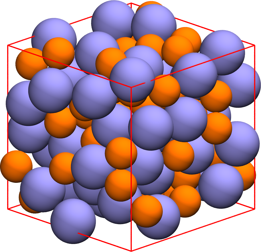
What does non-Gaussian mean?
What does non-Gaussian mean?
-
\( \alpha_2 = \frac{\left< x^4 \right> }{3 \left< x^2 \right> } - 1 \) is the "non-Gaussian parameter", used as a measure of dynamical heterogeneities
-
For a Gaussian distribution, \( \left< x^4 \right> = 3\left< x^2 \right> \), so \( \alpha_2 = 0 \)
-
Can be calculated from particle-tracking
What does non-Gaussian mean?
-
A random walk (diffusion) is Gaussian at any given time:
-
\( P(x, t) = \frac{1}{2 \sqrt{\pi D t}} - e ^ \frac{x^2}{4 D t} \)
-
-
So if the particles aren’t diffusing, then \( \alpha_2 \neq 0 \)
-
For caged particles, \( \alpha_2 \approx -\frac{1}{5} \)
-
-
Closely related to caging and cage-breaking behavior
-
In a cage, particles move very small distances
-
Cage-breaking would involve much larger jumps
-
The distribution of "step sizes" would be very non-Gaussian
-
What does non-Gaussian mean?
-
\( \alpha_2 \) measures how "not gaussian" the distribution is
Diffusion |
Mixed |
Caging |
\( \alpha_2 = 0 \) |
\( \alpha_2 > 0 \) |
\( \alpha_2 = -\frac{1}{5} \) |
Data
What kind of step distributions do we actually get?
What kind of step distributions do we actually get?
What kind of step distributions do we actually get?
The Non-Gaussian Parameter \( \alpha_2 \)
System Size Dependence of \( \alpha_2 \)
Lines drawn are \(A \left(\phi^\star - \phi\right)^n\), and \(\phi^\star \) is fitted
System Size Dependence of \( \alpha_2 \)
α₂ goes to ∞?
-
Provocative, but inconclusive
-
\( \phi^\star = 0.600 \pm 0.001\) is an unusual density
-
There is less than two orders of magnitude on this plot
-
3.5 is a long ways from ∞
-
Maximizing \( \alpha_2 \)
Maximizing \( \alpha_2 \)
-
Start with the sum of two gaussians \( P(r) \propto A r ^ 2 \sigma ^ 2 e ^ {-\frac{r ^ 2}{\sigma ^ 2}} + B r ^ 2 e ^ {-r^2} \)
-
Increasing σ while decreasing \( \frac{A}{B} \) gives a larger \( \alpha_2 \)
-
More specifically: For a given σ, \( \frac{A}{B} = \frac{\sigma ^ 2}{1 + \sigma^2} \) yields the maximum \( \alpha_2 = \frac{\left(\delta ^ 2-1\right)^2}{4 \delta ^2} \)
-
Back to the Step Distributions
-
As we increase density, we get an increased separation
-
As time varies, the ratio \( \frac{A}{B} \) varies
Approximating \( \alpha_2 \) with Aging
-
Prepare a state at \( \phi_0 = 0.55 \) at equilibrium
-
Fast quench it to some density \( \phi \)
-
Calculate \( \max_{\Delta t} \alpha_2 \) as a function of time
Aging \( \alpha_2 \)
Cartoon
|
Simulation
|
Close to Jamming
Close to Jamming

-
Glassy behavior starts at \( \phi \approx 0.55 – 0.59 \)
-
Jamming is at \( \phi \approx 0.64 \)
-
What happens if we go really close to jamming?
-
Permanent Caging
-
Floaters
-
Step Distributions Close to Jamming
Close to Jamming: |
Glassy: |
Peak at \( 10^{-2} \) : Tight Cages |
Peak at \( 10^{-1} \) : Caged Floaters |
Peak at \( 10^{-1} \) : Caged Particles |
Peak at \( 10^{0} \) : Rearrangements |
Step Distributions Close to Jamming
Solid: Backbone |
Dashed: Floaters |
Thin Dotted: Both |
Rearrangements
-
Each dot represents a single system
-
At 1000 timepoints over the course of the simulation, a snapshot was taken, and the structure was "minimized" to find the inherent structures visited
-
Systems seem able to access either a very limited number of inherent structures, or a very large number
Other Directions
Fitting The Step Distributions
-
Fit the step distributions to the sum of two gaussians
-
Figure out how that scales with time and ϕ
-
This is hard.
That’s all.
Thanks!
-
Corey O’Hern, Mark Shattuck, Christine Jacobs-Wagner
-
Brad Parry, Ivan Surovtsev, Eric Dufresne, and everyone I talked to
-
Sackler, PEB, and HHMI